Beyond the mean, median, and mode

[Thanks to Drake Thomas and Mike Winston for discussion.]

In third grade math class, my teacher Ms. Potter taught my class about the mean, median, and mode of a list of numbers. What united these numbers, Ms. Potter told us, was that they were measures of central tendency: numbers that represented, in some sense, the “middle” of the data.

I remember being dissatisfied with the mode being labeled a measure of central tendency. After all, it’s really easy to construct an example (1, 1, 2, 3, 4, …, 100) where the mode is nowhere close to the middle of the data. I don’t remember whether I voiced this objection to Ms. Potter, but my mental model of her would have responded with “Well, for typical lists of numbers that occur in real life, the mode generally is close to the middle” — or anyway, that’s the half-satisfying explanation I ended up giving myself.

But as pointed out by Buck Shlegeris, there is some really cool math connecting the mean, median, and mode, and the mode really does deserve its place as a measure of central tendency.

To re-explain Buck’s post: the median $m_1$ of a list of numbers is the number that minimizes the sum of the distances to the numbers in the list. Try thinking about why this is: take some list of numbers (of odd length, for simplicity) — 0, 1, 5, 20, 23, for example — and think about how the function $f_1(x)$ , defined as the sum of the distances from $x$ to each number, i.e. $f_1(x) = |x| + |x - 1| + |x - 5| + |x - 20| + |x - 23|$ , varies with $x$ . I think you’ll be able to convince yourself that $f_1(x)$ is minimized when $x = 5$ , and that this is the case precisely because $5$ is the median number in the list.

(For an even number of elements, there is a tie for this minimum value among all numbers in between the two middle numbers, inclusive — so for the list 0, 1, 5, 8, 20, 23, every number in the interval $[5, 8]$ could be considered the median, per this new interpretation of the median).

What about the mean? It turns out that the mean $m_2$ of a list is the number the minimizes the sum of the squares of the distances to the numbers in the list. One way to see this is, say your list of numbers is $x_1, \dots, x_n$ . We are looking for the minimum of $f_2(x) = |x - x_1|^2 + \dots + |x - x_n|^2$ . Taking the derivative with respect to $x$ , we find that $f_2$ is minimized when $\sum_i (x - x_i) = 0$ , which is true precisely when $x$ is the mean.

And the mode? It turns out that’s just the number $m_0$ minimizing $f_0(x) = |x - x_1|^0 + \dots + |x - x_n|^0$ (if we use the convention that $0^0 = 0$ ). That’s because $f_0(x)$ is equal to $n$ minus the number of times that $x$ appears in the list.

And so if you’re mathematically inclined, you’re probably thinking, why stop there? We can define $m_p$ (the p-median) of a data set to be the $x$ that minimizes $f_p(x) = |x - x_1|^p + \dots + |x - x_n|^p$ . The 0-median is the mode, the 1-median is the median, the 2-median is the mean… maybe other values of $p$ are interesting as well.

At this point in the post, if you’re so inclined, it would be a good time to pause and see what you can discover about p-medians for general values of $p$ (the case $0 < p < 1$ is probably most interesting) for yourself. Or if not, keep reading!

It turns out that when $0 < p < 1$ , the p-median of a list is always one of the numbers in the list! I made a GeoGebra file if you’d like to play around and get some intuition for why this is true. Here’s a formal argument: consider

$f_p(x) = \sum_i |x - x_i|^p$ .

Here’s a plot of $f_p(x)$ with the list [0, 2, 3, 5, 8, 11] for $p = 0.57$ :

Geogebra_Example

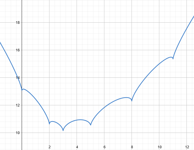
We have

$f_p''(x) = \sum_i p(p - 1)|x - x_i|^{p - 2}$

which is negative on each interval $(x_i, x_{i + 1})$ , meaning that $f_p$ is concave on each such interval (as you can see in the picture). Therefore the only possible minima of $f_p$ are at the points $x_i$ .

So, given a list, which values are the p-median for some $p \in (0, 1)$ ? Here’s an instructive example: consider the list

0, 1, 1, 3, 4, 5, 50, 60, 61, 62, 70, 80, 90.

The p-median changes with p as follows:

For $0.88 \le p \le 1$ , the p-median is 50 (the median).
For $0.68 \le p \le 0.87$ , the p-median is 60.
For $0.61 \le p \le 0.67$ , the p-median is 61.
For $0.54 \le p \le 0.6$ , the p-median is 4.
For $0.5 \le p \le 0.53$ , the p-median is 3.
For $0 \le p \le 0.49$ , the p-median is 1.

The key intuition here is that for p close to 1, the p-median is near the middle of the list. As p gets smaller, being close to other elements matters more and more. This makes sense, because the 0-median is the mode, i.e. the number in the list with the greatest number of other list members that are exactly equal to it.

In this example, several elements of the list are the p-median for some p; but it is no coincidence that 0 and 90 never are. Assuming that the smallest and largest elements of the list each appear only once, they can never be the p-median. To see that, take the smallest and second-smallest elements, and consider the distances from them to every other element in the list. In our earlier example [0, 1, 5, 20, 23], the distance from 0 to the other elements is 1, 5, 20, 23, and the distance from 1 to the other elements is 1, 4, 19, 22. Comparing these distances one by one, we find that the distances from the second-smallest elements are always smaller than the corresponding distances from the smallest element, meaning that for any p, the sum of distance raised to the p-th power is smaller for the second-smallest element than the smallest. This reasoning also works for the largest and second-largest elements.

Is it possible to have a list of numbers of arbitrary length such that every element besides the two extreme ones serves as the p-median for some $p \in (0, 1)$ ? This is a fun exercise; see this footnote for the answer.¹

Another question is: what’s the behavior of the p-median in the limit as p approaches 0? This is a cool question because it’s a natural way to define the mode of a list of distinct numbers. Recall that for $x$ close to zero, we have $e^x \approx 1 + x$ . This lets us write

$f_p(x) = \sum_i |x - x_i|^p = \sum_i e^{p \ln |x - x_i|} \approx n + p \sum_i \ln |x - x_i|$

for p close to 0, which means that the limiting value of $f_p(x)$ is the element of the list that minimizes the sum of the logs to the other elements. Equivalently, the mode of a list of distinct numbers is the number the product of whose distances to the other numbers is as small as possible. So for instance, the mode of the list 0, 1, 2, 3, 4, 5, 10, 11, 12, 13 is 3. It’s pretty cool that the mode generalizes so naturally!

This leads us to an interesting connection of the p-median with the generalized mean. The p-power mean of a list of nonnegative numbers $d_1, \dots, d_n$ is defined to be

$\left(\frac{1}{n} \sum_{i = 1}^n d_i^p\right)^{1/p}$ .

Familiar cases are the arithmetic mean ( $p = 1$ ), the quadratic mean/root mean square ( $p = 2$ ), the harmonic mean ( $p = -1$ ), and — interestingly — the geometric mean (the limit as p approaches 0).

The median (1-median) of a list of numbers is the number that minimizes the arithmetic mean (1-power mean) of the distances to the numbers in the list. The (arithmetic) mean (2-median) is the number that minimizes the quadratic mean (2-power mean) of the distances. The mode (0-median) minimizes the geometric mean (0-power mean) of the distances.² More generally, perhaps a more natural definition of the p-median is the number that minimizes the p-power mean of distances to the numbers in the list.

Indeed, this is the definition that extends naturally to negative values of p, allowing us to define the -1-median as the number maximizing the sum of the reciprocals of the distances to all other numbers.

What about the limit as p approaches infinity? As p grows to infinity, the p-median becomes the average of the smallest and largest numbers in the list, because large distances are punished more and more relative to smaller ones.

And as p approaches negative infinity? There, having small distances to one’s neighbors is increasingly rewarded, so the p-median becomes the number in the list with the smallest distance to its closest neighbor. (Well, there are two such numbers; it’s the one whose distance to its other neighbor is smaller.)

So as p varies, we observe some interesting behaviors:

When p is really large, the p-median is the average of the two extreme elements.
As p gets closer to 2, the p-median becomes more and more equally influenced by each element of the list (in the sense that perturbing each element has the same effect on the p-median).
As p further decreases to 1, the p-median approaches the middle value(s) of the list.
As p decreases toward and beyond 0, the p-median tends toward elements that are close to other elements. In the limit as p becomes very negative, being close to your nearest neighbor is the only thing that matters.

I see the p-median, for $p < 1$ , as a summary of the data which may be a reasonable choice under some circumstances. Let’s say you’re at a party and want to know the population of the United States, in millions. You ask around and get some guesses:

100, 320, 320, 325, 330, 400 (median), 500, 600, 700, 1000, 1500

But something interesting is going on in the data: four of the numbers are really close together. A reasonable conclusion to draw from this data set is that four of the people you asked know the approximate answer, while seven are just guessing. If I knew nothing about the population of the United States and saw these answers, I’d guess that the population is 325 million even though the median answer was 400 million (and the mean is even larger).

This is what the p-median accomplishes for $0 < p < 1$ : in its choice of a consensus, it balances clustering (detecting knowledge of the underlying matter) with moderation (looking for middle ground in a way that’s resistant to extreme answers). And indeed, as you decrease p from 1 to 0, around $p = 0.87$ the p-median switches from 400 to 330. Around $p = 0.75$ it switches to 325, and around $p = 0.57$ it switches to 320 (the mode).

So here’s a bold conjecture: in practice, when estimating quantities in the real world from asking around, using the 0.8-median is better than using the median.

I’m very uncertain in this conjecture –I’m not sure I’d bet on it at even odds (though it’s close) — but I find it very plausible and it would be very interesting if it were true.

^{1. Yes, it is possible! One example is (for arbitrary ). The idea is that when , the p-median (i.e. the median) is . As you decrease p, the p-median becomes more and more “mode-ish” (i.e. having lots of numbers close to yours matters more and more relative to being in the middle of the data). So as you decrease p, the p-median switches to numbers that are further and further form the median. You can easily modify this example to get lists of even length with the same property.↩}

^{2. Well technically that’s 0 for every number in the list, but the limit of the p-median as you push p to zero is the number minimizing the geometric mean of the distances to all other numbers.↩}

8 thoughts on “Beyond the mean, median, and mode”

Pingback: Beyond the mean, median, and mode (a generalization of medians) - Nevin Manimala's Blog
Rory O’Kane says:

February 16, 2020 at 2:29 am

Someone in a Reddit discussion of this post mentioned the concept “M-estimator”. The Wikipedia article on M-estimators is too dense for me to fully understand, but it does seem like they are related.

LikeLike

1. Eric Neyman says:
  
  February 16, 2020 at 6:44 am
  
  Thanks for the pointer! I wasn’t able to understand the article at first glance but will take a look again later 🙂
  
  LikeLike
  
Douglas Summers-Stay says:

May 9, 2020 at 11:32 am

I thought this was very interesting. What about data in more than one dimension? What are the best measures of central tendency for 2-D data, or 1000-D data?

LikeLike

1. Eric Neyman says:
  
  May 9, 2020 at 5:37 pm
  
  Good question (which I won’t answer)! As you point out, p-medians generalize to n dimensions; see e.g. https://en.wikipedia.org/wiki/Geometric_median. I would be quite interested to see if anyone has any cool observations about p-medians in higher dimensions!
  
  Another interesting thing to think about is p-medians for continuous distributions, rather than finite sets of numbers/points. It would be cool to draw some (asymmetric) distribution and then animate where the p-median is as p changes. (I don’t think I’m up to this task though.)
  
  LikeLike
  
gabrieldwu says:

August 14, 2021 at 12:56 am

Great work! I was actually thinking about this relationship between mean (minimizing squares) and median (minimizing first powers) a few months ago, but I never realized how you could also think of mode this way. It’s interesting how for negative p, the p-median is forced to be one of the numbers of the original list because it needs to be infinity plus some real value (and choosing a point that isn’t among the list would only have a finite value). You avoided dealing with infinity stuff by defining it to be one of the numbers and only looking at distances to other points, but it results to the same thing.

I’m also wondering if you have an intuitive way to see that the p-median has a unique value? Is it ever the case that there are two distinct values that, say, minimize the sum of fifth powers of distances to the numbers? I’m discounting special cases like mode, which can be a whole interval.

LikeLike

1. Eric Neyman says:
  
  August 14, 2021 at 4:57 am
  
  Yeah so I think that for any p > 1 this is true. That’s because for any $x_i$ , $(x - x_i)^p$ is strictly convex, which means that $\sum_i (x - x_i)^p$ is strictly convex, and a strictly convex function can only have one minimum.
  
  LikeLiked by 1 person
  
Pingback: A Few of My Favorite Links – Harsimony